Understanding Loops and Iterations in Python
Loops are a fundamental concept in programming that allows us to execute a set of instructions repeatedly until a specific condition is met. They are essential for automating repetitive tasks and solving complex problems more efficiently. In Python, loops are a crucial part of the language, and there are several ways to implement them.
The Need for Iterations
In mathematics and computer science, we often encounter problems that require a repetitive approach to reach a solution. This approach is known as “iteration.” It involves repeatedly applying a set of steps until a desired result is achieved. Let’s explore this concept further with an example.
The Guessing Game: Finding the Square Root
Suppose we want to calculate the square root of a number, such as 196. We can represent this problem as an equation:Copy code
x^2 = 196
Our objective is to find the value of ‘x.’ To keep things simple, we’ll focus on finding the positive square root.
Two things are evident about the solution:
- The square root is greater than 0.
- The square root is less than 196.
This information defines the range of our solution, which is from 0 to 196. To find the square root, we could start at 0 and increment our guess step by step until we arrive at the correct value.
A python loop for the solution will appear in the following manner:
| for _x in range(0,196,1): if (_x * _x) == 196: print("Square root of 196 is: ", _x) |
Now, let’s implement the square root guessing program in Python, which prompts the user to input a number and utilizes a loop to find the square root. (sqaure_root.py)
| square_root.py |
| # program to 'Guess' square root of a number # Ask for number for calculating square root _s = int(input("Enter number for calculating square root: ")) # loop for guessing, range 0 to _s, with step increase of 1 for _x in range(_s): if (_x*_x) == _s: print("Square root of ", _s, " is: ", _x) else: print(_s, " is not a perfect square") |
One key observation: the ‘range’ in the ‘for’ loop command is shortened
for _x in range(_s): instead of for _x in range(0, _s, 1):
Simplifying the Range
You may have noticed that we use for _x in range(_s) instead of the more detailed for _x in range(0, _s, 1).
In Python, when you don’t specify the starting point and step size, the default values are assumed to be 0 and 1, respectively. So, we can simply use range(_s) to achieve the same result.
The output for our program is as follows:
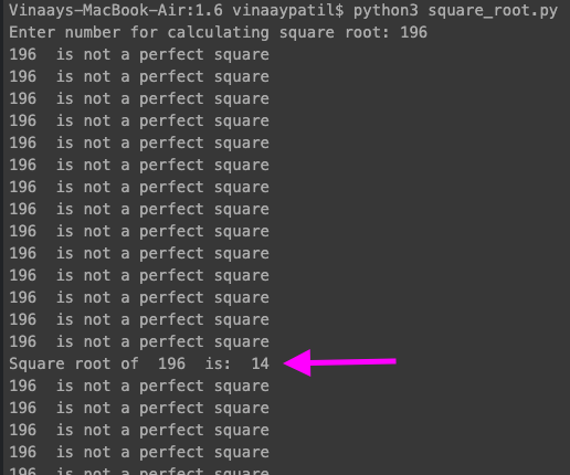
The output is quite absurd.
Analyzing the Output
Upon analyzing the output, we observe the following issues:
- Every time the ‘guess’ doesn’t match the solution, the program enters the “else” statement and prints that the input is not a perfect square. This occurs as we move from ‘0’ upwards (1, 2, etc.).
- When the ‘guess’ reaches the solution, the “if” condition is met, and it prints the square root. But the program doesn’t stop; it continues to the next step (15, 16, and so on) and once again enters the “else” statement.
To stop a loop midway, we have the ‘break’ command. Incorporating the above observations, let’s create an improved program. (improved_sqrt.py)
| improved_sqrt.py |
| # program to ‘Guess’ square root of a number # Ask for number for calculating square root _s = int(input(“Enter number for calculating square root : “)) # loop for guessing, range 0 to _s, step increase of 1 for _x in range(_s): if (_x*_x) == _s: print(“Square root of “, _s, ” is: “, _x) break if (_x*_x != _s): print(_s, ” is not a perfect square” |
The ‘break’ command is a signal for the program to exit the loop. We have given it within the ‘if’ condition. When the condition is met, i.e., we have our solution ( (_x*_x) == _s), then the ‘break’ command will ensure that further ‘guessing’ is stopped.
The improvements we’ve made are as follows:
- Moving the ‘else’ statement: We correctly identified that the ‘else’ statement should be executed after the ‘for’ loop. This ensures that it is only executed once the loop has exhausted all possible guesses and not during each iteration.
- Using the ‘break’ statement: We’ve effectively used the ‘break’ statement to exit the loop as soon as the solution is found. This prevents the loop from continuing unnecessarily.
With these changes, the program now behaves as expected and provides accurate results. Here’s what the program outputs
A much better execution.
Continue a loop until a specific condition is met.
In our previous program, we used a ‘for’ loop to continue until a certain condition was met, at which point we used the ‘break’ statement to exit the loop. This two-step process is effective, but Python offers a more concise alternative.
While Loop
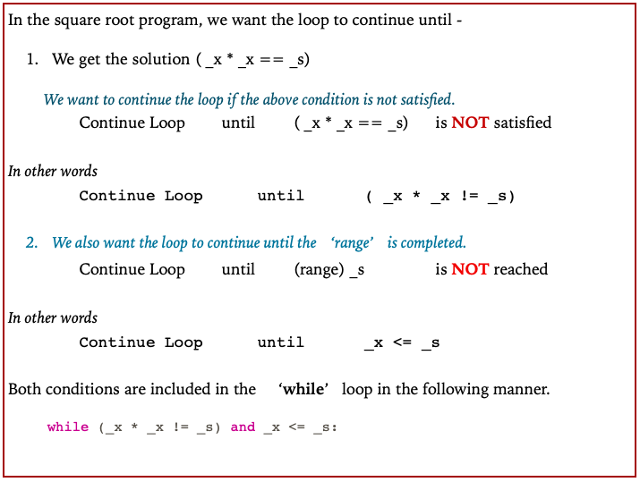
Python provides us with another type of loop, the ‘while’ loop, which combines both the looping condition and the exit condition into a single statement.
(! corresponds to ‘NOT’)
Compared to the ‘for’ loop the ‘range’ is not specified automatically. The ‘while’ loop specifies only the ‘end’ point. ( _x <= _s)
Thus, we have to specify both, the ‘start’ point and the ‘step size’ separately.
| While Loop Implementation |
| # Start point for the while loop _x = 0 # while loop while _x <= _s and (_x * _x != _s): _x = _x + 1 # Step size = increment of ‘1’ |
As an alternative to the ‘for’ loop, we can achieve the same goal using the ‘while’ loop. The ‘while’ loop is particularly helpful when we want to specify both the starting point and the step size within the loop. Let’s delve into how the ‘while’ loop works and explore its advantages.
Understanding the ‘while’ Loop
Compared to the ‘for’ loop, the ‘while’ loop differs in the way it handles the range. While the ‘for’ loop automatically specifies the starting point, step size, and end point, the ‘while’ loop only specifies the end point using a conditional statement. In other words, we need to define both the starting point and the step size explicitly.
Let’s see how we can implement the ‘while’ loop for our square root guessing program:
| while_sqrt.py |
| # program to ‘Guess’ square root of a number # Ask for number for calculating square root _s = int(input(“Enter number for calculating square root : “)) # Start point for the while loop _x = 0 # while loop for guessing the square root while (_x * _x != _s) and _x <= _s: _x = _x + 1 if (_x*_x == _s): print(“Square root of “, _s, ” is: “, _x) else: print(_s, ” is not a perfect square”) |
At an initial glance, the program will seem slightly odd. Only one operation occurs within the while loop ( _x = _x + 1), whereas all the remaining conditionality statements are outside the loop.
In this program, we set the start point for the ‘while’ loop by initializing _x to 0 before entering the loop. The ‘while’ loop is governed by the condition (_x * _x != _s) and (_x <= _s). As long as both conditions hold true, the loop continues to iterate, with each iteration incrementing _x by 1.
Algorithm
Let’s break down how the ‘while’ loop calculates the square root of 196:
STEP 1 : Declare and Initialize Variable
The variables have the following values: _s = 196 , and _x = 0
STEP 2 : First Iteration, check our conditions for solution
In the first iteration of the ‘while’ loop, we check the conditions: _x = 0
- Condition 1: _x * _x != _s (0 * 0 != 196)
- Condition 2: _x <= _s (0 <= 196)
Both conditions are satisfied, so we enter the loop, and _x is incremented to 1.
STEP 3 : While Loop Continues as long as conditions are met (till _x =13)
- The ‘while’ loop continues in the same manner, and the value of _x increases (1, 2, 3, 4, 5, and so on).
- After several iterations, we reach _x = 13.
- At this point, the conditions are still met, and we continue to increment _x.
STEP 4 : While Loop Breaks ( at _x=14)
- Finally, after numerous repetitions, we reach _x = 14.
- In the next iteration:
- Condition 1: _x * _x != _s (14 * 14 != 196)
- Condition 2: _x <= _s (14 <= 196)
- Condition 1 is not satisfied, so we exit the ‘while’ loop with the value of _x = 14.
STEP 5 : We exit the While Loop and Check which condition is met
- _x = 14.
- IF: _x * _x == _s (14 * 14 = = 196)
- We have found our answer
- ELSE:
- The number is not a perfect square
The ‘while’ loop essentially keeps iterating as long as both conditions are met, and it stops as soon as one of the conditions fails. This behavior allows us to find the square root efficiently.
The output for the program (while_sqrt.py) is as follows
When we run the ‘while’ loop program (while_sqrt.py), we observe no significant difference between the outputs from the ‘for’ loop and the ‘while’ loop. Both loops yield the same result.
(In case you are still not getting the feel on how the ‘while’ loop is getting executed, it might be a good idea to explore the program in ‘Thonny’ in step wise debug mode)
The Differences between the ‘two’ loops can be tabulated as below:
| No | For Loop with If | While Loop |
| 1 | # loop for guessing, range 0 to _s, step increase of 1 for _x in range(_s): if (_x*_x) == _s: print(“Square root of “, _s, ” is: “, _x) break | # Initialize for while loop _x = 0 # while loop for guessing the square root while _x <= _s and (_x *_x != _s): _x = _x + 1 |
| 2 | with range initial value of ‘0’
and step size of ‘1’ is automatically defined in ‘range’ option of the ‘For loop’ | initial value needs to be set before commencing the ‘while’ loop
_x = 0 Step size needs to be defined within the ‘while’ loop _x = _x +1 |
| 3 | A ‘break’ command is required to stop the loop when the ‘conditionality’ on ‘if’ is met | Loop automatically breaks when ‘conditionality’ within the ‘while’ loop is met |
| 4 | For each conditionality, separate ‘if’ commands are needed
for _x in range(_s): ……. if (_x*_x*_x) == _s ……. | Multiple conditionality statements can be added within ‘while’ loop by using ‘and’ ‘or’ statements
while _x <= _s and (_x *_x != _s) or (_x *_x*_x != _s) |
| 5 | for [iterating variable] in [sequence]:
[do something] | while [a condition is True]:
[do something] |
Up to this point, our square root guessing program has employed a ‘brute force’ approach. It systematically tries every available option one after the other until it reaches the answer. For instance, when finding the square root of ‘196,’ it took ’14’ steps to arrive at the result (starting from 1 and incrementing).
While this method may be convenient for smaller numbers, it becomes highly impractical when dealing with larger numbers. Consider an example like ‘19600,’ where the square root is ‘140.’ Using the ‘brute force’ method would require ‘140’ steps to reach the solution, making it significantly inefficient.
To expedite the process, we need a more intelligent technique instead of relying on blind guesses. One such method is the Bisection Method.
Enhancing Efficiency: The Bisection Method
In this method, the ‘guess’ is calculated using a formula called the ‘bisection’ formula.
The term ‘bisection’ means ‘to bisect’ or, in other words, ‘to split into two halves.’ In this method, the ‘guess’ is calculated using a formula known as the ‘bisection’ formula. Instead of a linear search as in the ‘brute force’ approach, the ‘bisection’ method narrows down the possibilities more efficiently.
Here’s how the Bisection Method works:
Our current Guess has divided our solution interval in two parts. We shall select a ‘New Interval’ for our next guess.
| Interval 01 | Guess | Interval 02 | |
| x | 0 – 9800 | 9800 | 9800 – 19600 |
| x2 | 96,040,000 | ||
| Comparing to solution | 96,040,000 > 19600 | ||
| Observation | Lower than current guess | ‘New Guess’ should be less than our current ‘Guess’ | Higher than current guess |
| New Interval | 0 – 9800 | Eliminated | |
| New Guess | (0 + 9800) /2 = 4900 |
Once we have a ‘New Guess’ we repeat the procedure over and over again (Iterations)
The general practice is to put a limit on the number of ‘iterations’ say ’10’ iterations or to stop when we get the solution.
Flowchart
We can implement the flowchart in the following program
| bisection.py |
| # Program to find square root using bisection # Get input for finding square root _s = float(input(“Enter number for calculating square root: “)) _limit = int(input(“Enter number of iterations: “)) # Define interval for initial solution _high = _s _low = 0.0 _iter = 0 _x = (_high + _low)/2 # Create loop with condition while (_x * _x) != _s and _iter < _limit: if (_x * _x) > _s: _high = _x else: _low = _x _iter = _iter+1 _x = (_high + _low)/2 print(“At”, _iter, ” iteration solution is: “, _x) print(“After “, _iter, ” iterations the square root of “, _s, ” is : “, _x |
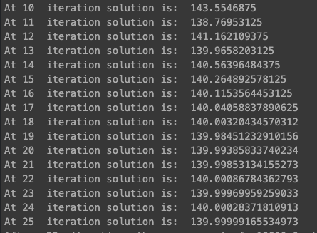
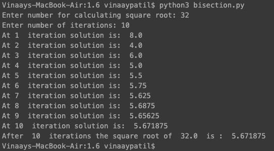
The output of the program is as follows
From the output of our program using the Bisection Method, a few important observations become evident:
The Use of Floats
- Advantage of Floats: One clear advantage of using ‘floats’ instead of ‘integers’ for our calculations is that, after the 3rd iteration, we enter the realm of decimal numbers. The square roots of many numbers are not whole integers, and it’s important to use ‘floats’ to accurately represent and calculate these decimal values.
The Bisection Method: An Approximation Technique
- Approximation Nature: The Bisection Method is inherently an approximation technique. As we increase the number of iterations, our solution becomes increasingly ‘closer’ to the actual value. For instance, at the end of 10 iterations, the calculated value is ‘143.554,’ with an error of 3.554 (|143.554 – 140|).
- Trade-off Between Accuracy and Time: There’s always a trade-off between the accuracy of the solution we desire and the time or number of iterations it takes to reach that solution. The Bisection Method allows us to control this trade-off. If we prioritize higher accuracy, we can increase the number of iterations, which will result in a more precise estimate. This is in contrast to the ‘brute force’ method, which would require significantly more steps to achieve a similar level of accuracy. For example if we take 25 steps, the answer has an error in the sixth decimal place.
Handling Non-Perfect Squares:
Another notable advantage of the Bisection Method is its ability to calculate the approximate roots of non-perfect squares. For instance, if we were to apply the ‘brute force’ method to the number ’32,’ it would inform us that ’32 is not a perfect square.’ However, when we provide ’32’ to the Bisection Method, it approximates the root as ‘5.671’ after 10 iterations. This showcases the flexibility of the Bisection Method in handling a wider range of cases, making it a valuable tool in numerical computation.
In summary, the use of ‘floats’ and the Bisection Method together offer a more accurate and flexible approach to calculating square roots. The Bisection Method’s approximation nature allows us to strike a balance between accuracy and efficiency, making it a powerful tool for numerical computations, especially when dealing with both perfect and non-perfect squares
Choice of Loop
Whether to use ‘for‘ loop or ‘while‘ loop is a matter of convenience. Whichever you find useful to get the desired output is acceptable.
The critical question is: Is ‘while‘ loop just an additional method to execute the same operations done by a ‘for’ loop?
The answer is ‘NO.’
While ‘for’ and ‘while’ loops can often be used interchangeably to achieve similar results, they have their own unique purposes. It’s important to be comfortable using both loops and to select the one that best fits the problem you’re solving.
In the context of the square root calculation programs we’ve explored, both ‘for’ and ‘while’ loops were used effectively. The ‘for’ loop provided a clear way to iterate through a known range, while the ‘while’ loop allowed us to iterate until a specific condition was met.
As we progress in our programming journey, we’ll encounter more situations that will make it evident when to use one type of loop over the other. Additionally, we’ll discover specific features of the ‘for’ loop, such as traversing lists and strings, which will be explored in later chapters.
Roots of Quadratic Equation using Python
Let’s consider an application of these techniques: finding the roots of a quadratic equation. Solving equations can present challenges, such as determining the range for solutions and handling both positive and negative roots.
For instance, consider the equation 2x^2 + 10x = 1288. To tackle equations like this, we can prompt for a range and account for both positive and negative roots.
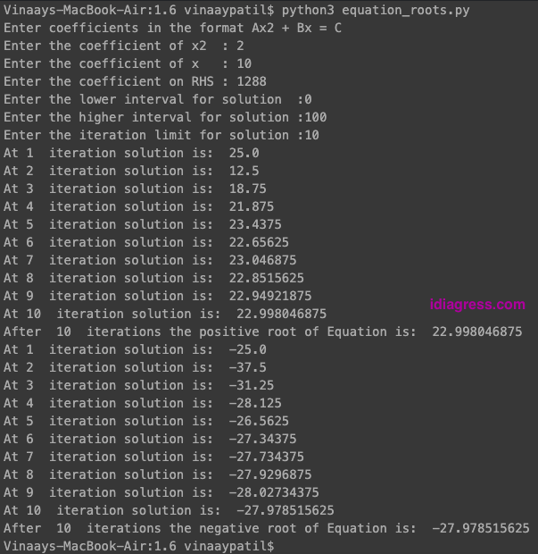
The program for finding the roots of a quadratic equation (equation_roots.py) is more extensive, but the underlying logic remains the same, relying on the Bisection Method implemented through a ‘while’ loop. The output is as follows.
For the equation 2x^2 + 10x = 1288, the real roots are x = 23 and x = -28. Our ‘bisection’ method provides approximate roots of x = 22.998 and x = -29.97.
These approximate roots are indeed quite close to the actual roots. It’s worth noting that the change in values during successive iterations is different for the positive and negative roots. This disparity emphasizes the robustness of the ‘bisection’ algorithm.
However, in hindsight, it becomes clear that there is room for improvement in our program. One aspect that could be enhanced is the inclusion of a statement to handle cases where the solution falls outside the specified interval. This adjustment would make the program even more robust and user-friendly.
Maybe you can improve the program accordingly.
Exercise
- Implement a program to calculate the cube root of a given number, using the brute force method in a ‘for’ loop.
- Implement the previous program using the ‘bisection’ method.
- Modify the program to calculate cube root using ‘bisection,’ to include a max permissible error to stop the loop.
| For example, |
| Number = 3375
Interval ( 0 to 3375), Limit on iterations (10), Max permissible error ( 0.1 ) So the loop should stop, either when the limit on iterations is reached, OR, if the answer falls between ( 14.9 to 15.1) while …… and …… or abs(_X**3 – _S) < 0.1: abs( ) returns the ‘absolute’ value of the operation. abs(14+9) = abs(23) = 23 abs(-14-9) = abs(-23) = 23 abs(-14+9) = abs(-5) = 5 Essentially it returns the ‘+ve’ value, and for ‘–ve’ values, if present, it is converted into a ‘+ve’ sign |
- Find the ‘fifth’ root of the number ‘537824’ using Bisection method
- Implement a program to find if the roots of equation 2x3 + 10x = 5628, lie in between -70 to 70.
In this chapter on Python loops and iterations, we’ve explored fundamental concepts related to loops, iteration, and the practical application of these concepts. Key points covered in this chapter include:
- Introduction to Loops: Loops are a fundamental programming concept used to execute a set of instructions repeatedly until a specific objective is achieved. We’ve seen how loops are essential for automating repetitive tasks.
- Iterations: Iterations involve repeating a set of steps until a desired solution is obtained. We’ve learned how iterations are fundamental in various computational and mathematical processes.
- ‘For’ Loop: We’ve explored the ‘for’ loop, a loop that iterates over a predefined range, making it suitable when the number of iterations is known in advance. The ‘for’ loop is commonly used to work with sequences like lists and strings.
- ‘While’ Loop: The ‘while’ loop continues to execute as long as a specified condition holds true. It provides flexibility when the number of iterations is not known beforehand and is useful for scenarios that require continuous condition checking.
- The Bisection Method: We’ve introduced the Bisection Method, an approximation technique used to narrow down solutions efficiently. This method involves dividing the solution space into two parts and iteratively refining the guess to achieve a desired level of accuracy.
- Using Floats and ‘While’ Loops: We discussed the advantages of using ‘floats’ for precise calculations and highlighted the ‘while’ loop’s suitability for visualization of conditionality in a single line.
- Efficiency and Trade-offs: We’ve explored how the Bisection Method offers a trade-off between accuracy and the number of iterations. Increasing the number of iterations improves precision but may require more time.
- Application: Finding Roots of Quadratic Equations: To apply these concepts, we solved quadratic equations using the Bisection Method and presented a program to find the roots of a given equation. We discussed the program’s strengths and identified areas for potential improvement.
The chapter has equipped you with foundational knowledge of loops and iterations, introduced the Bisection Method as a powerful approximation technique, and demonstrated practical applications of these concepts. As you continue to explore Python programming, you’ll have a solid foundation to build upon and adapt these concepts to a wide range of problem-solving scenarios.









[…] Prev Chapter Course Homepage Next Chapter […]
[…] Prev Chapter Course Homepage Next Chapter […]