


Moving on from our exploration of quadratic equation roots, we are about to dive into another captivating realm of problem-solving.
Yet, before we do, it’s essential to acknowledge a limitation in our bisection program. Our current implementation works well for cases with one positive and one negative root.
However, it falls short when both roots share the same sign, be it positive or negative. To illustrate, let’s consider the equation (x+2)(x+5), which expands to x^2 + 7x + 10. In this scenario, the roots are x = -2 and x = -5, both negative. Unfortunately, our current program captures only one of these two roots.

From the Output, it is clear the program needs work. Maybe you can work and try to improve it.
For now, let’s move to Factorization
A. Prime Factorization
In mathematics, factors of a number are those values that, when multiplied together, yield the original number. For instance, in the case of 24, we can express it as the product of 12 and 2. Here, 12 and 2 are factors of 24.
Nonetheless, in mathematical pursuits, our primary concern lies in discerning the prime factors of a number. Prime factors are those indivisible components of a number that are prime themselves. For example, when we delve into the prime factors of 24, we can decompose it into 2, 2, 2, and 3—a collection of purely prime factors.
Let’s now delve into crafting an algorithm for the precise determination of these prime factors.
Here’s a step-by-step approach to finding the prime factors of a number:
- Start with the number you want to find the prime factors of (let’s call it
n). - Initialize an empty list to store the prime factors.
- Begin with the smallest prime number, which is 2.
- Check if
nis divisible by 2. If it is, add 2 to the list of prime factors and dividenby 2 repeatedly until it is no longer divisible by 2. - Move on to the next prime number, which is 3, and check if
nis divisible by 3. If it is, add 3 to the list of prime factors and dividenby 3 repeatedly until it is no longer divisible by 3. - Continue this process, incrementing the prime number each time, and checking if
nis divisible by the current prime number. If it is, add the prime factor to the list and dividenby that prime number as many times as possible. - Repeat steps 4-6 until you have exhausted all prime numbers less than or equal to the square root of
n. After this, ifnis greater than 1, it means thatnitself is a prime factor. - You now have a list of prime factors that, when multiplied together, will give you the original number
n.
The fundamental idea behind prime factorization is to progress through the sequence of prime numbers (2, 3, 5, 7, 11, and so on) until the quotient becomes ‘1.’
Now, you might wonder if it’s necessary to maintain a list of all prime numbers. Interestingly, besides ‘2,’ all prime numbers are ‘odd.’ Therefore, a more efficient approach is to simply advance through the list of odd numbers. This simplifies the programming.
But what about factors that are ‘odd’ yet not ‘prime’? For instance, consider 27, which can be expressed as 9 multiplied by 3. The factor ‘9’ in this case is ‘not a prime’ number. The primary goal, however, is to isolate prime numbers.
Here’s a crucial point to grasp: By starting with a lower odd number (e.g., 3) and continually dividing until reaching a non-zero remainder, we effectively eliminate non-prime factors before encountering a non-prime number.
To illustrate, let’s take the number 99 as an example. Our concern is the possibility of capturing a non-prime factor. In this instance, 99 can be factored into 9 and 11. But what if ‘9’ is mistakenly identified as a factor?

We can see that the factor of ‘9’ gets reduced before we reach ‘9’ as a divisor. Thus, it does not get captured as a factor
This greatly simplifies our program. We don’t need to maintain a list of prime numbers; we can move upwards without worrying about non-prime numbers getting captured as factors.
Flow of the program
| Step No | Command | Interpretation | Paramater Value | |
| 1 | _number = int(input(“Enter the number for factorization:”)) | Ask user to input value of number for factorization | _number = 132 | |
| 2 | while _number % 2== 0: | 2 is a factor till remainder is zero | 132 % 2 = 0 TRUE | |
| 2.L.1 | print(“2 is a factor”) | |||
| 2.L.2 | _number = _number / 2 | Get quotient | _number = 132/2
_number = 66 | |
| while _number % 2== 0: | 2 is a factor till remainder is zero | 66 % 2 = 0 TRUE | ||
| 2.L.1 | print(“2 is a factor”) | |||
| 2.L.2 | _number = _number / 2 | Get quotient | _number = 66 /2
_number = 33 | |
| while _number % 2== 0: | 2 is a factor till remainder is zero | 33 % 2 = 0 FALSE | ||
| EXIT WHILE LOOP | ||||
| 3 | for _fac in range(3, _number, 2): | begin ‘for’ loop to scan for ‘odd’ factors NOTE: We are jumping range by ‘2’, which means we will go, 3, 5, 7, i.e ODD numbers. | _fac = 3
_number = 33 | |
| 3.L.1 | while _number % _fac== 0: | _fac is a factor till remainder is zero | 33 % 3 = 0 TRUE | |
| 3.L.2 | print(_fac, “ is a factor”) | |||
| 3.L.3 | _number = _number / _fac | Get quotient | _number = 33 /3
_number = 11 | |
| 3.L.1 | while _number % fac == 0: | _fac is a factor till remainder is zero | 11 % 3 = 0 FALSE | |
| EXIT WHILE LOOP | ||||
| _fac in range(3, _number, 2) | _fac = _fac + 2
range increment | _fac = 3 + 2
_fac = 5 | ||
| 3.L.1 | while _number % fac == 0: | _fac is a factor till remainder is zero | 11 % 5 = 0 FALSE | |
| EXIT WHILE LOOP | ||||
| _fac in range(3, _number, 2) | _fac = _fac + 2
range increment | _fac = 5 + 2
_fac = 7 | ||
| 3.L.1 | while _number % fac == 0: | _fac is a factor till remainder is zero | 11 % 7 = 0 FALSE | |
| EXIT WHILE LOOP | ||||
| _fac in range(3, _number, 2) | _fac = _fac + 2
range increment | _fac = 7 + 2
_fac = 9 | ||
| 3.L.1 | while _number % fac == 0: | _fac is a factor till remainder is zero | 11 % 9 = 0 FALSE | |
| EXIT WHILE LOOP | ||||
| _fac in range(3, _number, 2) | _fac = _fac + 2
range increment | _fac = 9 + 2
_fac = 11 | ||
| 3.L.1 | while _number % _fac== 0: | _fac is a factor till remainder is zero | 11 % 11 = 0
TRUE | |
| 3.L.2 | print(_fac, “ is a factor”) | |||
| 3.L.3 | _number = _number / _fac | Get quotient | _number = 11 /3
_number = 1 | |
| 3.L.4 | fac in range(3, _number, 2) | FINISH program as _fac is beyond range | _fac > _number
11 > 1 |
Based on the above algorithm the program (basic_factors.py) is as follows:
| basic_factors.py |
| _number = int(input(“Enter number for Factorization: “)) while _number % 2 == 0: print(“2 is a factor “) _number = _number /2 for _fac in range (3, _number, 2): while _number % _fac ==0: print(_fac, ” is a factor”) _number = _number/ _fac |
The output of the program is as follows.
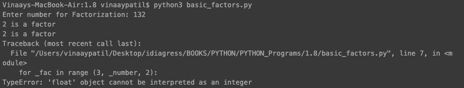
The output successfully executes the code for the first ‘while’ loop, identifying ‘2’ as a factor. However, a challenge arises when the program enters the ‘for’ loop, resulting in an error related to a ‘float’ object.
This issue stems from the fact that during the process of dividing a number, the data type can transition to ‘float.’ For instance, when we execute the operation _number = _number / 2, _number becomes a ‘float’ data type.
The problem arises when we subsequently pass this variable, which is now a ‘float,’ into the ‘range’ function. It’s crucial to note that the ‘range’ function exclusively accepts ‘integer’ variables, and this discrepancy leads to the error..
To circumvent this issue, we need to reconvert the variable back to an ‘integer’ before using it in the ‘for’ loop. We can achieve this by applying the following modification:
for _fac inrange (3, int(_number), 2):This alteration ensures that the data type of _number remains as an ‘integer’ within the ‘for’ loop, preventing any ‘float’ object errors. This refined approach maintains data type consistency and facilitates accurate prime factorization.

B. Comparison of Factors
In our existing program, we are proficient at identifying factors of a given number. However, what’s currently missing is the mechanism to store these factors. Since our objective is to collect all the factors in one organized place, the most practical approach is to employ a ‘list.’
We can leverage the append() function to conveniently add identified factors to a list. To achieve this, we will encapsulate the steps for calculating factors within a dedicated function and return a list containing all the factors for a specified number.
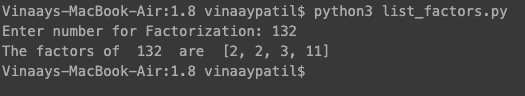
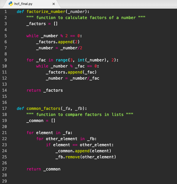
The program, titled ‘list_factors.py,’ is structured as follows:
| list_factors.py |
| def factorize_number(_number): “”” function to calculate factors of a number “”” _factors = [] while _number % 2 == 0: _factors.append(2) _number = _number/2 for _fac in range(3, int(_number), 2): while _number % _fac == 0: _factors.append(_fac) _number = _number/_fac return _factors _a = int(input(“Enter number for Factorization: “)) _factors_a = factorize_number(_a) print(“The factors of “, _a, ” are “, _factors_a) |
We’ve carried out a straightforward replacement in the code. Wherever in our previous program, there was a print("is a factor"), we’ve replaced it with _factors.append to add the identified factor to a list. The result is a neatly organized list of factors.
The next part will be to factorize two numbers, so that we can calculate the H.C.F. (Highest Common Factor).
Let’s see a sample HCF calculation.
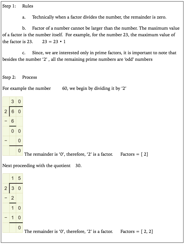
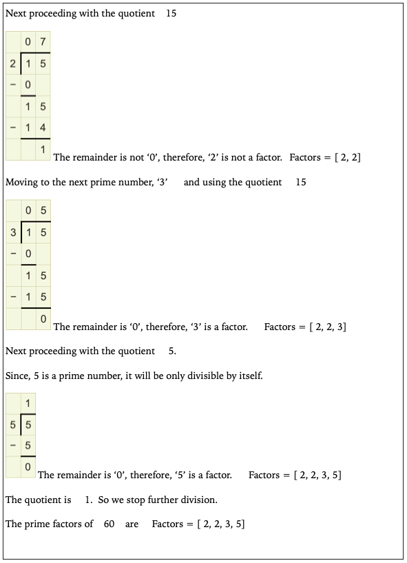
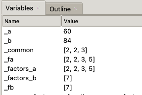
Calculate HCF of the numbers 60 and 82
Factors of 60 are [ 2 , 2 , 3 , 5 ]
Factors of 84 are [ 2 , 2, 3 , 7 ]
Comparing the factors and highlighting common factors
[ 2, 2, 3 , 5 ] [ 2, 2, 3 , 7 ]
Common factors are [ 2 , 2 , 3 ]
HCF is multiplication of common factors = 2 • 2 • 3 = 12
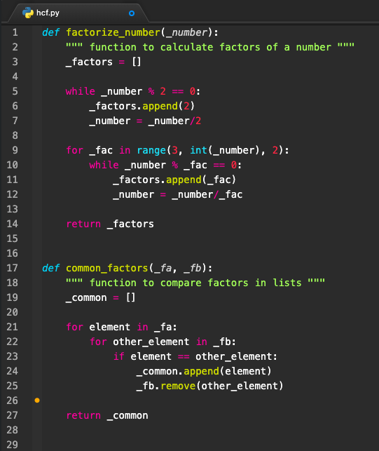
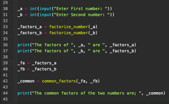
Our program excels at calculating the factors and storing them in a list. The next essential task is to compare these two lists and construct a new list comprising all the common factors.
To accomplish this comparison, we iterate through the elements of list A and, for each element, check against every other element in list B. If two elements match, we add that element to a common list and ensure it isn’t considered again in subsequent comparisons. The logic for this comparison can be expressed as follows:
| For every | element | in | list A, |
| we want to check every | other element | in | list B, |
| and | if the two elements are equal | add element in | a Common list |
| Plus, | Don’t consider the element again | in the | next comparison |
Code wise we can write the logic as:
| Appending function for Factors |
| for element in _fa: for other_element in _fb: if element == other_element: _common.append(element) _fb.remove(other_element) return _common |
We now need to code the above code for comparison as a function defined to compare two lists.
The program (hcf.py) is as follows.
The output is

C. Immutable and Mutable
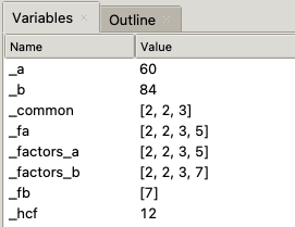
Before we delve into our program and calculate the HCF by multiplying the common factors, it’s crucial to grasp a fundamental concept about lists and other data types: the distinction between mutable and immutable objects. To gain a clearer understanding, you can run your program in Thonny or insert print commands in the Atom file to examine the final values of variables.
If you scrutinize the final values of variables, you’ll observe that the list _factors_b has been modified from [2, 2, 3, 7] to [7]. This modification takes place even after we saved _factors_b in _fb before passing the lists into the functions. Both lists are being altered within the function.
This behavior can be attributed to the fact that, in Python, everything is an object, and objects are categorized into two groups: mutable and immutable.
- Mutable Objects: These are objects whose values can change. When you modify a mutable object, it alters the object itself. Lists and dictionaries are examples of mutable objects.
For instance, if you have a list _a = [2, 3, 5, 7, 11] and another list _b = _a, both _a and _b point to the same object in memory. Modifying one list will affect the other because they share the same object.
- Immutable Objects: These are objects whose values do not change once they are created. Numbers and strings are examples of immutable objects.
For instance, if you have an integer a = 5 and another integer b = a, both a and b are distinct objects with the same value. Modifying one will not affect the other.
In the context of our program, when we copied _factors_b to _fb, both variables were essentially referencing the same list object, which is why modifications to one list were reflected in the other.
On the other hand, for mutable objects, the object’s name points to an address in memory. Thus when we copy an immutable object, we do not create a new object. We simply create another name that points to the same address. Thus, change one, and the copy also changes. Lists and Dictionaries are mutable.
To resolve this, we can use the copy() function when duplicating lists. This function creates a distinct copy of the list, ensuring that changes made to one list do not impact the other.
 Instead of  _fa = _factors_a,
we can use _fa = _factors_a.copy()
This creates an independent copy of the list.
In addition to this modification, we’ll also add another function to multiply the factors and obtain the HCF in the program (hcf_final.py).

The output is as follows

And when we check out the variables, we see that the original lists are preserved.
Now, here comes a pivotal question: Is it truly necessary to preserve these lists of factors? In this case, the resounding answer is “Yes!”
This necessity becomes evident when you consider the typical progression in mathematical problem-solving. After calculating the Highest Common Factor (HCF), the subsequent task often revolves around determining the Least Common Multiple (LCM). The LCM is, essentially, the result of multiplying the common factors with the non-common factors.
Mathematically speaking, the LCM is defined as:
LCM = Common Factors • Non-common Factors
Hence, to accurately calculate the LCM, you must have access to the original factor lists once again. These lists are indispensable for distinguishing between the common and non-common factors, a critical step in finding the LCM.
As an exercise create a program to calculate LCM
Summary
we have explored the process of factorization, which involves breaking down a number into its prime factors. This process is essential for various mathematical calculations, including finding the Highest Common Factor (HCF) and the Least Common Multiple (LCM) of numbers.
Here’s a summary of the key points covered in this chapter:
- Factorization: Factorization is the process of breaking a number down into its prime factors, which are the indivisible components of the number.
- Prime Factors: Prime factors are prime numbers that multiply to form the original number. They are crucial for various mathematical calculations.
- Algorithm for Finding Prime Factors: We discussed an algorithm for finding the prime factors of a number, which involves iterating through prime numbers and dividing the number until it becomes 1.
- Storing Factors in Lists: We learned how to store the identified factors in lists for easy access and further calculations.
- Mutable and Immutable Objects: Understanding the concept of mutable and immutable objects is vital. Immutable objects, like numbers and strings, retain their values when copied, while mutable objects, like lists, can change when copied.
- Preserving Lists: We emphasized the importance of preserving the original lists of factors, especially when calculating the LCM, which depends on both common and non-common factors.
Overall, this chapter has laid the foundation for efficient mathematical problem-solving by providing tools and insights into factorization, the use of lists, and the significance of distinguishing between mutable and immutable objects in Python.


