


In our ‘Bisection’ program designed to calculate the roots of a quadratic equation, we have identified a specific issue. It appears that our program functions correctly when one root is positive and the other is negative. However, when both roots are either positive or negative, our program does not perform efficiently. This situation is technically referred to as a ‘bug’ within the program.
A ‘bug’ in coding occurs when the program fails to execute its intended purpose. These bugs typically fall into two categories. The first type results from errors in the program’s syntax, such as missing functions or incorrect usage. Syntax errors become evident during program execution. For instance, in a previous chapter, we encountered an error where the ‘range’ option within a ‘for’ loop required an ‘integer’ input, but we mistakenly provided a ‘float.’
Such errors are usually discovered while running the program, and we rectify them by modifying the code to ensure smooth execution. In essence, we eliminate the ‘bug’ from the code through a process commonly known as ‘debugging.’
The second type of ‘bug’ is more critical and relates to flaws in the program’s logic. In these cases, the program runs without any syntax errors, and Python does not report errors. However, due to faulty logic, the program’s output is incorrect. Our bisection program issue falls into this category.
To identify logic-related bugs, we typically conduct multiple ‘tests.’ These tests should encompass a wide range of real-world scenarios to comprehensively evaluate the program. For example, when testing our Highest Common Factor (HCF) program, we should consider various cases:
- Testing with two even numbers.
- Testing with two odd numbers.
- Testing with one even and one odd number.
- Testing with two prime numbers.
- Testing with one prime and one non-prime number.
The more rigorous and diverse the set of ‘tests’ we conduct, the more robust our program will become. Therefore, it is essential to thoroughly evaluate and validate our code by running extensive test cases. This practice ensures that our programs perform reliably and accurately. Now, let’s run some test cases on our HCF program to further enhance its functionality.
| No | Description | Test | Expected Output (HCF) |
| 1 | Two even numbers | 6 and 14 |
2 |
| 2 | Two odd numbers | 9 and 15 |
3 |
| 3 | One even, one odd number | 12 and 21 |
3 |
| 4 | Two prime numbers | 7 and 11 |
1 |
| 5 | One prime and one non prime number | 23 and 32 |
1 |

From the Output, it is evident that we have some misses.
| No | Test | Expected Output (HCF) | Python Output (HCF) |
| 1 | 6 and 14 |
2 |
2 |
| 2 | 9 and 15 |
3 |
3 |
| 3 | 12 and 21 |
3 |
1 |
| 4 | 7 and 11 |
1 |
1 |
| 5 | 23 and 32 |
1 |
1 |
The program is performing well in most cases, with only Test case 3 producing an incorrect output. Achieving a success rate of 4 out of 5 test cases, or roughly 80%, indicates the program’s overall effectiveness.
To analyze the error in Test case 3, we must scrutinize our program more closely. In our HCF program, we follow these steps:
- Factorize the given numbers.
- Identify common factors between the numbers.
- Multiply the common factors to calculate the HCF (Highest Common Factor).
The issue may lie within the third step, as we are not obtaining the expected result in Test case 3. To resolve this, we should:
- Review the factorization process to ensure that it correctly finds all factors of the numbers.
- Carefully examine the identification of common factors to verify that the program accurately identifies them.
- Double-check the multiplication of common factors to determine whether there is an error in this calculation.
By going through each of these steps and verifying their accuracy, we can pinpoint the source of the problem in Test case 3 and implement the necessary adjustments to improve the program’s performance. This process will help us achieve a higher success rate and ensure that the HCF program works effectively for all scenarios.
| No | Test | Step 1
Expected Output (Factors) | Step 1
Python Output | Step 2
Expected Output (Common) | Step 2
Python Output | Step 3
Expected Output (HCF) | Step 3
Python Output |
| 1 | 6 and
14 | [2, 3]
[2, 7] | [2]
[7] | [2] | [2] |
2 |
2 |
| 2 | 9 and
15 | [3, 3]
[3, 5] | [3, 3]
[3, 5] | [3] | [3] |
3 |
3 |
| 3 | 12 and
21 | [2, 2, 3]
[3, 7] | [2, 2]
[3, 7] | [3] | [ ] |
3 |
1 |
| 4 | 7 and
11 | [7]
[11] | [ ]
[ ] | [ ] | [ ] |
1 |
1 |
| 5 | 23 and
32 | [23]
[2,2,2,2,2] | [ ]
[2,2,2,2,2] | [ ] | [ ] |
1 |
1 |
It’s clear from the detailed analysis that our program, which initially appeared to be 80% effective, is in fact only 20% effective, and the correct values obtained were mostly due to luck. The root of the problem lies in the first step of the program, where it fails to capture the last factor in most cases. This issue becomes particularly apparent when dealing with prime numbers, where the single factor (the number itself) is not correctly identified.
To debug this error, Thonny is a useful tool. You can run the entire program step by step in Thonny, which allows you to understand why the last factor is being missed. In Thonny, you can use the “Debug script (nicer)” option, followed by “Step Into (F7)” to trace through the code and identify the problem.
For instance, in the very first test case, while factorizing the number ‘6’, we observe the following:
- Expected Output (Factors): [2, 3]
- Python Output (Step 1): [2]

We can see in the local variables, we have captured the first factor _factors = [2]
The _number variable is reduced to ‘3’
and since ‘3’ is a prime number, it should get captured. However, the range option the upper limit on the range is int(_number) i.e. int(3)
It appears that the issue with the program lies in the range used to find factors. In the specific case you’ve described, where the number ‘3’ is a prime number, the program fails to capture it as a factor due to the range’s upper limit being set to int(_number), which results in the range (3, 3, 2).
This range essentially doesn’t contain any values between 3 and 3, and as a result, the program doesn’t identify ‘3’ as a factor. To address this issue and ensure that prime numbers and the last factors are correctly captured, you should adjust the range limit in your code
Thus the full ‘range’ is (3, 3, 2) shown below
One way to handle this is to modify the range upper limit so that it includes the number itself. You can use int(_number) + 1 as the upper limit to ensure that the range covers all potential factors, including the number itself. Here’s how the code might look with this adjustment::
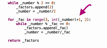
We increased the value of the upper limit on the ‘range’ by ‘+1’
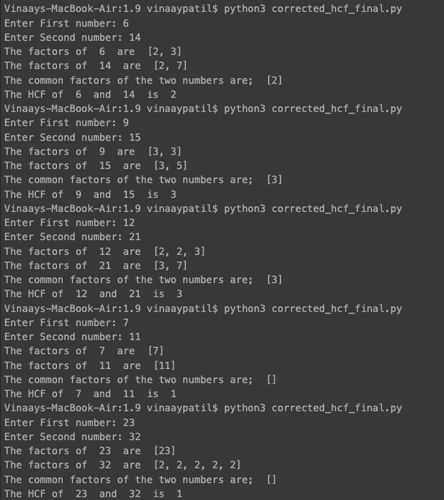
Testing it again. The output of the ‘corrected_hcf_final.py’ is as follows
| No | Test | Step 1
Expected Output (Factors) | Step 1
Python Output | Step 2
Expected Output (Common) | Step 2
Python Output | Step 3
Expected Output (HCF) | Step 3
Python Output |
| 1 | 6 and
14 | [2, 3]
[2, 7] | [2, 3]
[2, 7] | [2] | [2] |
2 |
2 |
| 2 | 9 and
15 | [3, 3]
[3, 5] | [3, 3]
[3, 5] | [3] | [3] |
3 |
3 |
| 3 | 12 and
21 | [2, 2, 3]
[3, 7] | [2, 2, 3]
[3, 7] | [3] | [3] |
3 |
1 |
| 4 | 7 and
11 | [7]
[11] | [7]
[11] | [ ] | [ ] |
1 |
1 |
| 5 | 23 and
32 | [23]
[2,2,2,2,2] | [23]
[2,2,2,2,2] | [ ] | [ ] |
1 |
1 |
Now, the solution is correct at all the steps, including the final Output.
What we saw here was Software Testing in action. Defining test cases, Running those tests, Identifying problem areas, Locating the problematic code, Re-testing, and repeating the cycle till we obtain the desired results
Summay
- Identifying Bugs: The chapter begins by explaining that a “bug” in programming refers to a situation where the program doesn’t execute its intended purpose.
- Types of Bugs: It categorizes bugs into two types. The first type is related to syntax errors, such as incorrect usage of functions or variables. The second type involves logical errors where the program runs without syntax errors, but the output is incorrect due to faulty logic.
- Thorough Testing: Thorough testing is essential to ensure that the program performs as expected. Various test cases are presented, and it’s emphasized that test cases should encompass real-world scenarios to comprehensively evaluate the program’s functionality.
- Debugging Process: The chapter discusses the debugging process, which involves running the program step by step to identify and rectify errors. The use of tools like Thonny for debugging is recommended.
- Problematic Code: It illustrates how to trace errors in code and provides an example where the program fails to capture the last factor in factorization, particularly for prime numbers.
- Adjusting the Range: The solution involves adjusting the range in the code to include the number itself, ensuring that all factors are correctly captured, including prime numbers.
- Software Testing in Action: The chapter concludes by highlighting the importance of software testing and how it involves defining test cases, running tests, identifying issues, locating problematic code, re-testing, and iterating until the desired results are achieved.
In summary, the chapter underscores the critical role of testing and debugging in software development, providing insights into how to systematically identify and resolve issues in the code, ultimately leading to more reliable and effective programs.
B. Working with external Files
Up to this point, both our program and its output have been confined to our software environment, typically within the Atom Terminal or Thonny’s Shell window. However, it’s important to note that this output is temporary. While the original code is stored as a ‘.py’ file on our computer, the output does not persist. This means that each time we wish to check the Highest Common Factor (HCF) of, let’s say, ‘6’ and ’14’ using our HCF program, we must open the code file and rerun it. Alternatively, we might resort to capturing a screenshot of the output and storing it as an image.
It would greatly enhance convenience if we could preserve the program’s output in a separate file. This way, whenever we need to reference the output, we can simply open the file without the need to re-execute the entire code.
The simplest way to achieve this is by writing the output to a ‘.txt’ file, which can be opened in any text editor.
To accomplish this, we must first instruct Python to create a ‘.txt’ file to store the output. Let’s assume that we want to create a file named ‘hcf_results.txt’ to contain the results.
_store = open(“hcf_results.txt”, ‘w’)
The syntax is as follows
_Nick_Name = open(“File_Name.txt”, ‘w – short for write‘)
We provide a nickname to the file, allowing us to access it directly using the nickname instead of specifying the full file path each time.
In Python, we use the open() function to work with files. Inside this function, we specify the name of the file in which we want to store the results, such as “results.txt.”
The open() function provides an option, denoted by a character, to define the file’s mode of operation. In this case, we use the ‘w’ option, which is short for ‘write.’ This indicates that we want to write values into the ‘results.txt’ file.
Other commonly used options include:
- ‘a’ for ‘append’: Used when you want to add data to an existing file.
- ‘r’ for ‘read’: Used for reading data from a file.
We will explore the usage of these other options in more detail as we proceed.
Once we have successfully opened the external ‘.txt’ file, we can write directly into it using the ‘print’ command. In the ‘print’ command, we specify the ‘txt’ file using the nickname we assigned earlier, which is typically denoted as (file = _store). This enables us to efficiently add content to the external file, such as our results.
print(“The HCF of “, _a, ” and “, _b, ” is “, _hcf, file=_store)
Python then directs the Output to an external file instead of the output shell window. Once we complete the ‘print’ commands, the last Step is to close the file using the close( )
_store.close()
The sequence of actions for working with an external ‘.txt’ file in Python can be summarized as follows:
- Open a text file in Python and give it a user-defined nickname or identifier.
- Incorporate a reference to the text file in the ‘print’ command using the assigned nickname (e.g.,
, file=nickname). - After writing to the file or performing operations, close the file to ensure data integrity and proper handling (e.g.,
nickname.close()).
By following these steps and utilizing the available options, here is what our program will look like (Note: The functions themselves are not detailed here but are assumed to be the same as in ‘corrected_hcf.py’):
output_hcf.py
_a = int(input(“Enter First number: “))
_b = int(input(“Enter Second number: “))
_factors_a = factorize_number(_a)
_factors_b = factorize_number(_b)
print(“The factors of “, _a, ” are “, _factors_a)
print(“The factors of “, _b, ” are “, _factors_b)
_fa = _factors_a.copy()
_fb = _factors_b.copy()
_common = common_factors(_fa, _fb)
print(“The common factors of the two numbers are; “, _common)
_hcf = multiply_factors(_common)
_store = open(“hcf_results.txt”, ‘w’)
print(“The HCF of “, _a, ” and “, _b, ” is “, _hcf, file=_store)
_store.close()
Most of the program remains the same, except the last three lines, wherein we have added the reference to the external ‘txt’ file. The Output is as follows

The last line is missing in the Output because we have diverted it to the ‘txt’ file. The ‘txt’ file’s location is the same folder from where we have executed our program. This reminds us (chapter 1.1) about organizing files in folders for good database management.
The external file, ‘results.txt’ is as follows.

As we can see, the results are in a separate ‘txt’ file, which we can access directly.
C. Input from CSV Files
Just as we can export program output to an external file, it’s equally convenient to import values from an external file. Let’s consider a scenario: suppose we want to calculate the Highest Common Factor (HCF) for five different sets of numbers, similar to our test cases. Currently, we would need to run our program five times to obtain the results. However, it would be much more convenient if we could store all our test cases in a single file and import them when needed.
When dealing with values stored in an external file, a simple ‘txt’ file won’t suffice. We need a way to distinguish one value from another within the file. This is where a CSV (Comma-Separated Values) file comes into play.
A CSV file is a type of file format designed for storing data, with values separated by commas. The name itself makes its purpose clear. In a CSV file, values are organized and separated by commas, enabling a structured and organized representation of data. This format is particularly well-suited for our test cases, and it allows us to define our test cases as follows:
6,14
9,15
12,21
7,11
23,32
And the good thing is that we don’t need a special editor to create this file. We can use the same text editor like ‘Notepad’ or ‘Atom’ to create this file. Just save the file as a ‘.csv’ file.

Before importing a CSV file in Python, it’s essential to plan for the fact that we need to calculate the Highest Common Factor (HCF) five times. We have two primary options for accomplishing this:
- Running the Program Multiple Times: We can run the program five times, each time providing different input data for the HCF calculation.
- Convert HCF Calculation into a Function: Alternatively, we can create a dedicated HCF calculation function and call it five times with different sets of input values. This approach is more structured and efficient.
The second option, which involves creating an HCF function, is the straightforward and recommended approach. The program’s structure will look something like this

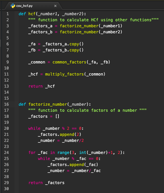
It is an overarching function (HCF function) calling other functions (Factorize, Common, Multiply) within it. The code for the function is as follows —
| def hcf(_number1, _number2): “”” function to calculate HCf using other functions””” _factors_a = factorize_number(_number1) _factors_b = factorize_number(_number2) _fa = _factors_a.copy() _fb = _factors_b.copy() _common = common_factors(_fa, _fb) _hcf = multiply_factors(_common) return _hcf |
Using this function we can create a simplified program.
| _a = int(input(“Enter First number: “)) _b = int(input(“Enter Second number: “)) _h = hcf(_a,_b) print(“The HCF of “, _a, ” and “, _b, ” is “, _h) |
(Note: we have defined all the functions before the above code)
Our next challenge is that the values of ‘_a’ and ‘_b’ should be automatically read from the ‘CSV’ file.
The first command we need to give is to inform Python that we can import a ‘CSV’ file. The command is straightforward.
import csv
Once we have indicated that we are opening a ‘CSV’ file, we now need to point to the specific file we want to import. We achieve this by using the with open ( ) syntax as follows
import csv
with open(‘test_cases.csv’, ‘r’) as csv_file:
n the with open() syntax for reading a CSV file, there are a few important considerations:
- File Location: You don’t need to specify the full path of the CSV file if it’s located in the same folder as your Python program. If the file is in a different directory, you would need to provide the complete file path to access it.
- File Mode: When reading from a file, as opposed to writing, you should use the ‘r’ option, which stands for ‘read.’ This option allows you to read the contents of the file.
After addressing these points, you can proceed to nickname the file and read its contents. The following code snippet illustrates how to do this:
| import csv with open(‘test_cases.csv’, ‘r’) as csv_file: csv_inputs = csv.reader(csv_file) |
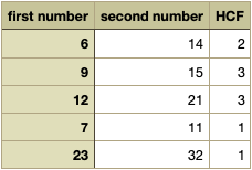
‘csv_inputs’ is the nickname. The csv.reader( ) function reads the contents of CSV file . The contents of the ‘CSV’ file are read in a ‘row-wise’ manner. The indexing is as follows.
| Row No | First entity | Delimiter | Second entity |
| 1 | 6 |
, |
14 |
| 2 | 9 |
, |
15 |
| 3 | 12 |
, |
21 |
| 4 | 7 |
, |
11 |
| 5 | 23 |
, |
32 |
| Index No |
[0] |
[1] |
Technically, the ‘comma’ is termed as a ‘delimiter’ and is ignored while indexing.
So, In ‘row 1’ ‘index 0’ is Row1[0] = 6
similarly, Row5[1] = 32
We can use the ‘for’ loop to go through the lines, and use the ‘index’ numbers to differentiate the variables.
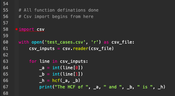
| import csv with open(‘test_cases.csv’, ‘r’) as csv_file: csv_inputs = csv.reader(csv_file) for line in csv_inputs: _a = int(line[0]) _b = int(line[1]) |
Adding our newly created HCF function within the ‘for’ loop will do the trick of repeating the calculation till the end of the ‘CSV’ file.
| import csv with open(‘test_cases.csv’, ‘r’) as csv_file: csv_inputs = csv.reader(csv_file) for line in csv_inputs: _a = int(line[0]) _b = int(line[1])_h = hcf(_a,_b) print(“The HCF of “, _a, ” and “, _b, ” is “, _h) |
The full program is as follows (csv_hcf.py)

The output of the program is as follows

this program, all calculations are performed directly without any direct input from us. The values from the CSV file are imported and used seamlessly for the calculations, making the process highly efficient.
To enhance this program, we can consider two options for storing the results:
- Printing Results in an External ‘txt’ File: By using a combination of the ‘open’ and ‘print’ commands, we can write the results to an external text file. This makes it easy to reference the results in a human-readable format.
- Exporting Output as a ‘CSV’ File: For even greater utility, we can export the output as a ‘CSV’ file. This format is advantageous because it can be easily imported into tools like ‘Excel’ for further analysis and visualization. To achieve this, we’ll need to create and open another ‘CSV’ file to store the output.
Both options have their advantages, and the choice between them depends on your specific needs and the preferred way of accessing and utilizing the program’s results.
with open(‘test_results.csv’, ‘w’) as csv_output_file:
Observe, we are using the ‘w’ option to indicate we want to write into this file.
Once again, Nick Naming the file, but this time with csv.writer ( ) function
import csv
with open(‘test_results.csv’, ‘w’) as csv_output_file:
res_file = csv.writer(csv_output_file)
To add a row in the ‘csv’ file we use the writerow( [ ] ) function. The function needs both curved and square brackets in the defination.
import csv
with open(‘test_results.csv’, ‘w’) as csv_output_file:
res_file = csv.writer(csv_output_file)
res_file.writerow([‘first number’,‘second number’,‘HCF’])
In the first row, we have given names to the entities that will come in the subsequent lines. To finalize we will add writerow( [ ] ) function within the ‘for’ loop.
The modified file (export_csv_hcf.py) will be as follows :
| # All function definations done # Csv import begins from here import csv with open(‘test_cases.csv’, ‘r’) as csv_file: csv_inputs = csv.reader(csv_file) with open(‘test_results.csv’, ‘w’) as csv_output_file: res_file = csv.writer(csv_output_file) res_file.writerow([‘first number’, ‘second number’, ‘HCF’]) for line in csv_inputs: _a = int(line[0]) _b = int(line[1]) _h = hcf(_a, _b) res_file.writerow([_a, _b, _h]) |
In the fame folder, we will now find a new file created — ‘test_results.csv’. We can import the file in Excel or similar software for further processing. We can see that in Excel, the data gets imported and neatly arranged in columns.
Summary
So far, we have covered several key concepts related to working with external files and enhancing the functionality of a Python program:
- Exporting Output: We discussed the importance of exporting program output to an external file for easy reference. This helps to store and retrieve results without rerunning the program.
- Importing Data: We explored the idea of importing values from an external file, specifically CSV files, for use in program calculations.
- File Location and Modes: We learned that when working with files, you don’t need to specify the full path if the file is in the same directory as your program. We also discussed the use of file modes (‘w’ for write and ‘r’ for read) to specify the intended operation.
- CSV Files: CSV (Comma-Separated Values) files were introduced as a structured way to store data with values separated by commas. This format is suitable for organizing test cases and other structured data.
- Reading CSV Files: We covered the process of reading CSV files using the
csv.reader()function. The data is read row-wise, and you can access values within each row using indexing. - Storing Results: We discussed options for storing program results. You can either print them to an external text file for human-readable access or export them as a new CSV file for further analysis in tools like Excel.
These concepts have demonstrated how to work with external files, import data, and enhance the functionality of a Python program by efficiently managing input and output
Exercise
- Create a program that takes input from a csv file of student names and their weight, and as an output delivers the average weight
- Create a program that creates a dictionary of usernames and password, and stores the values in a csv file
- Use the program created in step 2, to identify the longest password in the data
- Create a program to identify how many numbers in a csv file are prime numbers
- Create a program that calculates the cube root of a number and debug it using different scenarios
Best of luck
What Next
Another crucial aspect to consider is that a Python program is driven by the desired output format. You should always think about what format you want your program to produce. Not all steps or information need to be printed in the output; it’s essential to include only the relevant ones. For instance, in the HCF program, the CSV file that can be imported into Excel contains only three entities: the two numbers and the calculated HCF.
Throughout this course, the objective has been to familiarize you with the Python environment. By now, you should realize that Python programming primarily involves logical thinking and problem-solving. It’s essential to grasp that any code, regardless of its complexity, requires rigorous testing to make it foolproof. Without adequate testing and debugging, some issues may persist.
During testing and debugging, it’s crucial to break down the program into stages. This approach allows you to pinpoint the specific stage at which an issue arises, making it easier to identify and correct problems.
As a programmer, you should also be well-versed in different data types, such as integers, floats, lists, dictionaries, and more. Knowing how to switch between variable types and select the right one for a particular task is fundamental.
One of the key reasons to become familiar with Python is its widespread use. Python is integral to fields ranging from Machine Learning in Artificial Intelligence to Data Analytics in Big Data. Many software applications are built on Python’s foundation. While there are other specialized languages like “R” for specific tasks, you’ll often find that the logic underlying these languages is similar to Python.
In short, Learning Python, Practicing Python, simply makes sense!


No Comment